Functions

1)Round off a number.
ROUND(Value,places)
Function: Used to round off the value in a cell.
Arguments: Value is the actual value to be rounded off. Places is the number of decimals to round off to.

2)Square root of a number
SQRT(Value)
Function:Used to get the square root of the number
Arguments: Value is the actual number to be square rooted.

3)Round off the square root of a number
ROUND(SQRT)
Function: To Round off the square root of a number.
Arguments of Round:
Value: SQRT of the number is this case
Places: Number of decimals to be rounded off to.
Arguments of SQRT:
Value to be square rooted.

4)Minimum and Maximum of either 2 numbers or n numbers.
OR
Minimum and Maximum of a range of numbers.

UseCase 1:
Min(Value1,Value2,Value3,...valuen) Max(Value1,Value2,Value3,..valuen) This will give you the min or max value between the entered values

UseCase 2:
Min(CellM:CellN) Max(CellM:CellN) This will give the min or max of the values from a given range of values.

5)Ranking your data points.
Rank(Value, Range,Is_Ascending)
Function: Used to rank the data against a given range of values.
Arguments:
Value:Value to be ranked
Range/Data: Value to be ranked on the range of data
Is_Ascending: If set to 1 it will rank the data in an ascending order else Descending order
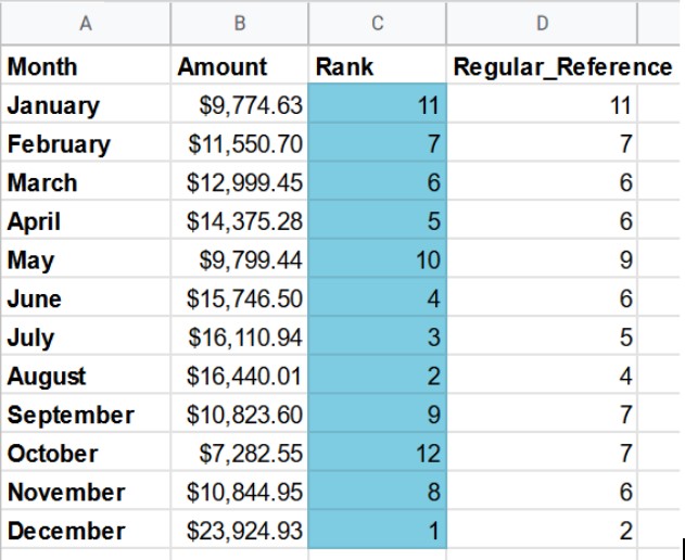
Important note:
We need to use the absolute reference here and not the regular one.
Regular: =RANK(B2, B2:B13)
Absolute=RANK(B2, $B$2:$B$13) This is because in the regular reference the end of the range (B13) is getting incremented and hence giving an unintended result.

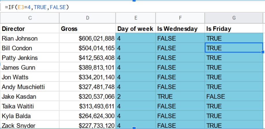
6)Conditional IF statement
Function: Used to write an if statement.
IF(Logical_expression,Value_if_true,Value_if_False)
Arguments:
Logical expression: Condition to be tested
Value_if_true: If the condition is true then the value to be given out
Value_if_false: This is the value to be given for the else part

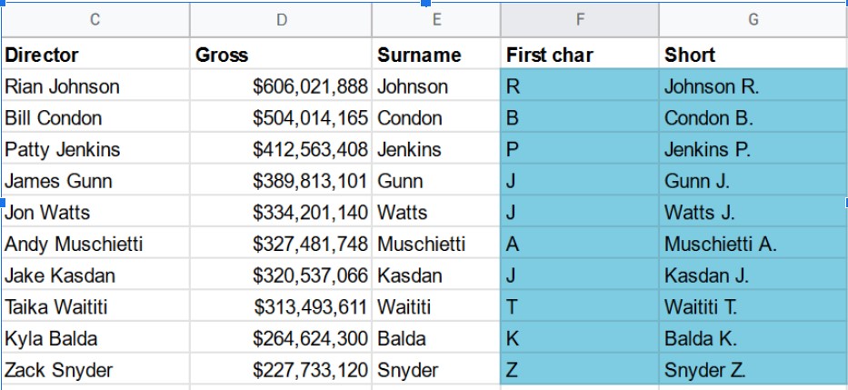
7)String Manipulation:

• LEFT(string, [number_of_characters]): selects the leftmost part of a string. The number of characters selected is defined in the optional argument number_of_characters, and defaults to 1.
  
  RIGHT(string, [number_of_characters]): selects the rightmost part of a string. The number of characters selected is defined in the optional argument number_of_characters, and defaults to 1. String information - LEN, SEARCH
  
  
• LEN(text): evaluates to the number of characters of text. E.g. =LEN("Cell") would evaluate to 4.
  
  SEARCH(search_for, text_to_search): searches for search_for in text_to_search:
  
  search_for: the string to look for
  
  text_to_search: the string to look in SEARCH evaluates to a number, the location in the string where search_for appears, with 1 being the first character.
  E.g. =SEARCH("e", "test test") would evaluate to 2, because the first "e" appears as the second character.
  
  Use len, search left, right to find the first name last name of the director.

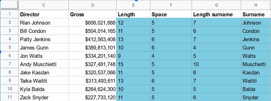
You can also do it in one go using: = RIGHT(C2, LEN(C2) - SEARCH(" ", C2))

8)Combining strings - CONCATENATE
How to combine strings using the CONCATENATE function:
CONCATENATE(string1, [string2, ...]): combines one or more strings into a single string.
E.g. =CONCATENATE("foo", " ", "bar") evaluates to foo bar.

9)Date functions - WEEKDAY
Some functions are used to get specific information or do operations on dates. One example of such a function is WEEKDAY: WEEKDAY(date, [type]): evaluates to the day of the week of a date. type is 1, 2 or 3.

type = 1: Sunday is day 1 and Saturday is day 7 (default)
type = 2: Monday is day 1 and Sunday is day 7
type = 3: Monday is day 0 and Sunday is day 6

For example, using =WEEKDAY(A1, 2) (where A1 contains the date 2019-01-01) would evaluate to 2, because January 1st 2019 fell on a Tuesday and setting type to 2 sets Monday at 1.

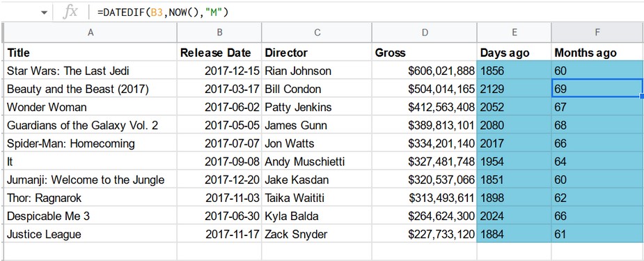
10)Comparing dates
Sometimes you might need to compare certain dates to each other, or to the current date. There are some useful functions for that in Google Sheets as well:
DATEDIF(start_date, end_date, unit): calculates the time difference between two dates. The difference will be calculated between start_date and end_date. The end_date must take place after the start_date. A third argument here is the unit, this can be:
"Y": the number of years between two dates
"M": the number of months between two dates
"D": the number of days between two dates

A full list can be found here NOW(): a function without arguments, evaluates to the current time
For example, =DATEDIF("2018-01-01", "2018-01-03", "D") would evaluate to 2.

SOURCE: DATACAMP course on spreadsheets

Go to next chapter